
How LLMs Actually Work: Transformers in 20 Minutes

Updated: 2 days ago

UIT University 365 Institute of Technology
Series AI Foundations | Level Basic (Free)
Duration 15 to 20 minutes | Access Free
IT Engineering, AI and Applied AI, Data Science, Software Development, Digital Transformation

UNOP Sound (University 365 Neuroscience Oriented Pedagogy)
Take five minutes to prepare your brain. Play the isochronous tone track (40Hz gamma frequency) with your eyes closed. Gamma-frequency tones before a learning session raise attention and make the material easier to absorb.
[Audio player: UNOP Pre-Lecture Isochrone (40Hz, 5 minutes)]
Table of Contents
The Hook: Your Question, Answered
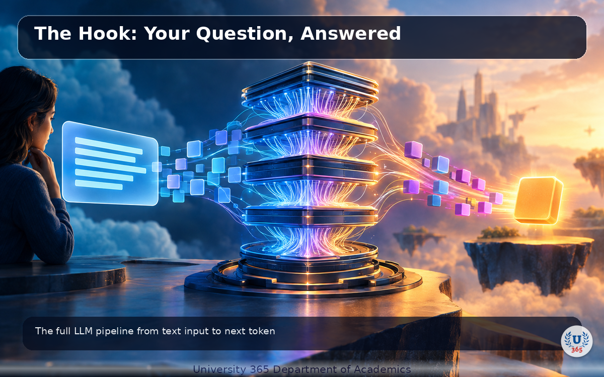
You type a question into ChatGPT. One second later, it responds with a coherent, relevant answer. What just happened?
In that second, your text traveled through a stack of mathematical operations called a transformer. The transformer processes every word simultaneously, lets each word "look at" every other word to understand context, and then predicts what word should come next. It repeats this prediction loop until the answer is complete.
The transformer architecture, introduced in 2017 by Google researchers in the paper "Attention Is All You Need," is the single most important innovation in modern AI. Every major language model (GPT-4o, Claude, Llama, Gemini, Mistral) uses it. Understanding the transformer is the foundation for everything else in AI engineering.
In the next 20 minutes, you will understand exactly what happens inside that one-second gap between your question and the answer.

Step 1: Tokenization: Breaking Text Into Pieces
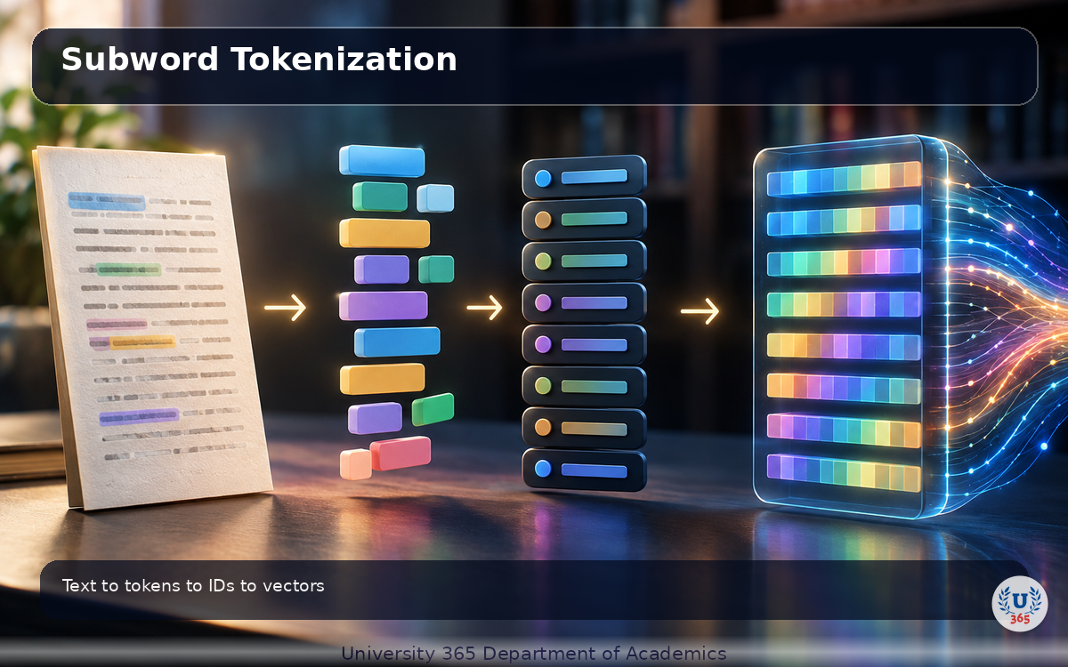
Language models cannot read text. They process numbers. The first step is tokenization: splitting your text into smaller pieces called tokens and converting each token into an integer ID.
How It Works
You write: "The cat sat"
The tokenizer splits this into tokens: ["The", " cat", " sat"]
Each token gets a unique ID from the model's vocabulary: [464, 3797, 3329]
Subword Tokenization
Modern models use Byte Pair Encoding (BPE), which breaks words into subword units. This handles rare words and misspellings without needing an enormous vocabulary:
"unbelievable" becomes ["un", "believ", "able"] (3 tokens)
"tokenization" becomes ["token", "ization"] (2 tokens)
Common words stay as single tokens: "the" = 1 token
BPE starts with individual characters and iteratively merges the most frequent adjacent pairs into new tokens until the target vocabulary size is reached. GPT-4 uses approximately 100,000 tokens. Llama 3 expanded to 128,000, which dramatically improved its ability to handle code and multilingual text with fewer tokens per input.
Why It Matters
Tokenization is a two-way map. The model must be able to decode tokens back to the exact original text. If any information is lost here, the model starts with a handicap it can never recover from. Tokenization also determines how much text fits in the model's context window: fewer tokens per word means more content fits.
Step 2: Embedding: From Numbers to Meaning
A token ID like 464 tells the model *which* token this is, but says nothing about what it *means*. The embedding layer fixes this. It is a lookup table where each token ID maps to a vector of real numbers (typically 4,096 to 16,384 dimensions).
How It Works
Token ID 464 (the word "The") maps to a vector like:
[0.050, -0.014, 0.065, 0.015, -0.023, ...] (4,096 numbers)
In a trained model, tokens with similar meanings have vectors that point in similar directions. "king" and "queen" are close. "king" and "apple" are far apart. The model learns these positions during training.
Positional Encoding
There is a problem: the vector for "cat" is identical whether it appears first or last in a sentence. But position matters. "The cat chased the dog" and "The dog chased the cat" mean very different things.
The solution is positional encoding: adding a unique position pattern to each token's embedding. The original transformer used sine and cosine waves at different frequencies. Position 0 gets one pattern, position 1 gets another, and so on.
Modern models like Llama use Rotary Position Embeddings (RoPE), which rotate the query and key vectors by an angle tied to their position. RoPE handles long texts better than sinusoidal encoding and has become the standard for frontier models.
What the Model Sees
After embedding and positional encoding, the model has a matrix of shape (sequence_length, embedding_dimension). For a 100-token input with a 4,096-dimensional model, that is a 100 x 4,096 matrix of real numbers. This matrix is the raw material that the transformer blocks will process.
Step 3: Self-Attention: How Tokens Talk to Each Other
This is the heart of the transformer. Self-attention lets every token look at every other token and decide how much to care about each one.
The Problem It Solves
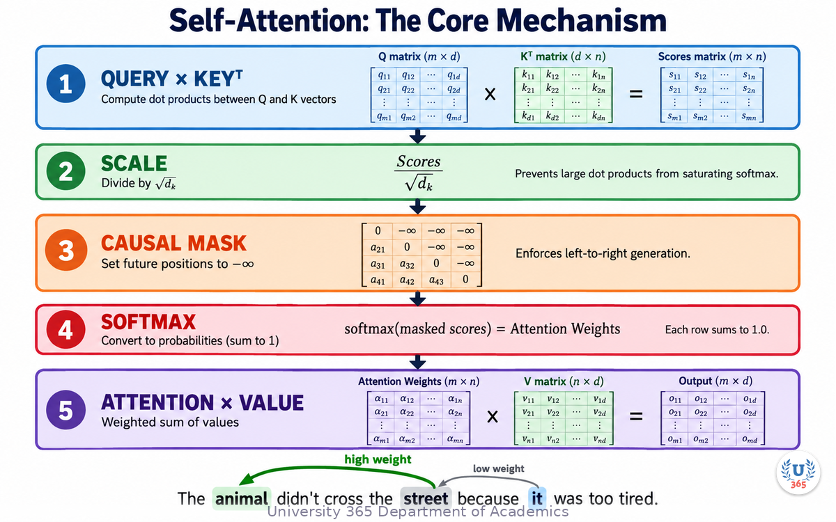
Consider: "The animal didn't cross the street because it was too tired."
What does "it" refer to? The animal or the street? A human knows instantly. An algorithm needs a mechanism to figure it out. Self-attention is that mechanism.
Query, Key, Value
Each token's vector gets projected three times using learned weight matrices:
Query (Q): "What am I looking for?"
Key (K): "What do I have?"
Value (V): "What information do I carry?"
The Attention Calculation
Score: Take the dot product of the query vector for one token with the key vector of every other token. High dot product means strong relevance.
Scale: Divide by the square root of the key dimension. This prevents the dot products from growing too large, which would push the softmax function into a flat zone with vanishing gradients.
Softmax: Convert the scaled scores into a probability distribution. Each weight is between 0 and 1, and all weights for one token sum to 1.
Weighted sum: Multiply each token's value vector by its attention weight and sum them up. This produces the attention output for that position.
The formula: Attention(Q, K, V) = softmax(QK^T / sqrt(d_k)) * V
What Happens with "it"
When processing "it", the query vector for "it" has high dot product with the key vector for "animal" (they are related in this context) and low dot product with "street". The softmax weights reflect this. The output for "it" is mostly a blend of "animal"'s value vector with a small contribution from "street". The model has resolved the reference.
Causal Masking
For text generation, a token can only look at tokens that came *before* it. Seeing future tokens would be cheating. This is enforced with a causal mask: a lower-triangular matrix that sets future positions to negative infinity before softmax. Softmax converts negative infinity to zero, so those tokens contribute nothing. This is why language models generate text left to right, one token at a time.
Step 4: Multi-Head Attention: Many Perspectives at Once
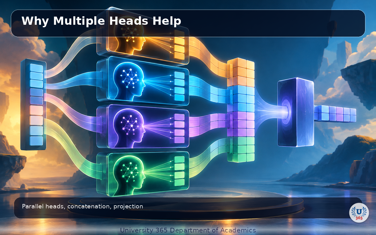
One attention head captures one type of relationship. But language has many types of relationships simultaneously: grammar, meaning, coreference, tone. Multi-head attention runs several attention computations in parallel, each with its own Q, K, V weight matrices.
How It Works
The original transformer used 8 heads
Modern models like Llama 3 70B use 64 heads
Each head operates on a slice of the embedding dimension (head_dim = embedding_dim / num_heads)
Each head can learn a different relationship type
The outputs of all heads are concatenated and projected back to the original dimension using a learned output matrix
Why Multiple Heads Help
One head might learn to track which noun owns which verb. Another might track which adjective modifies which noun. A third might track long-range coreference like "it" referring to "animal" three clauses back. Together, they capture richer patterns than any single head could.
Modern models use Grouped-Query Attention (GQA), which shares key and value heads across multiple query heads. This reduces the memory and computation cost of the attention mechanism during inference without significantly degrading quality. Llama 3 uses 8 KV heads shared across 64 query heads.
Step 5: The Transformer Block: The Repeating Unit
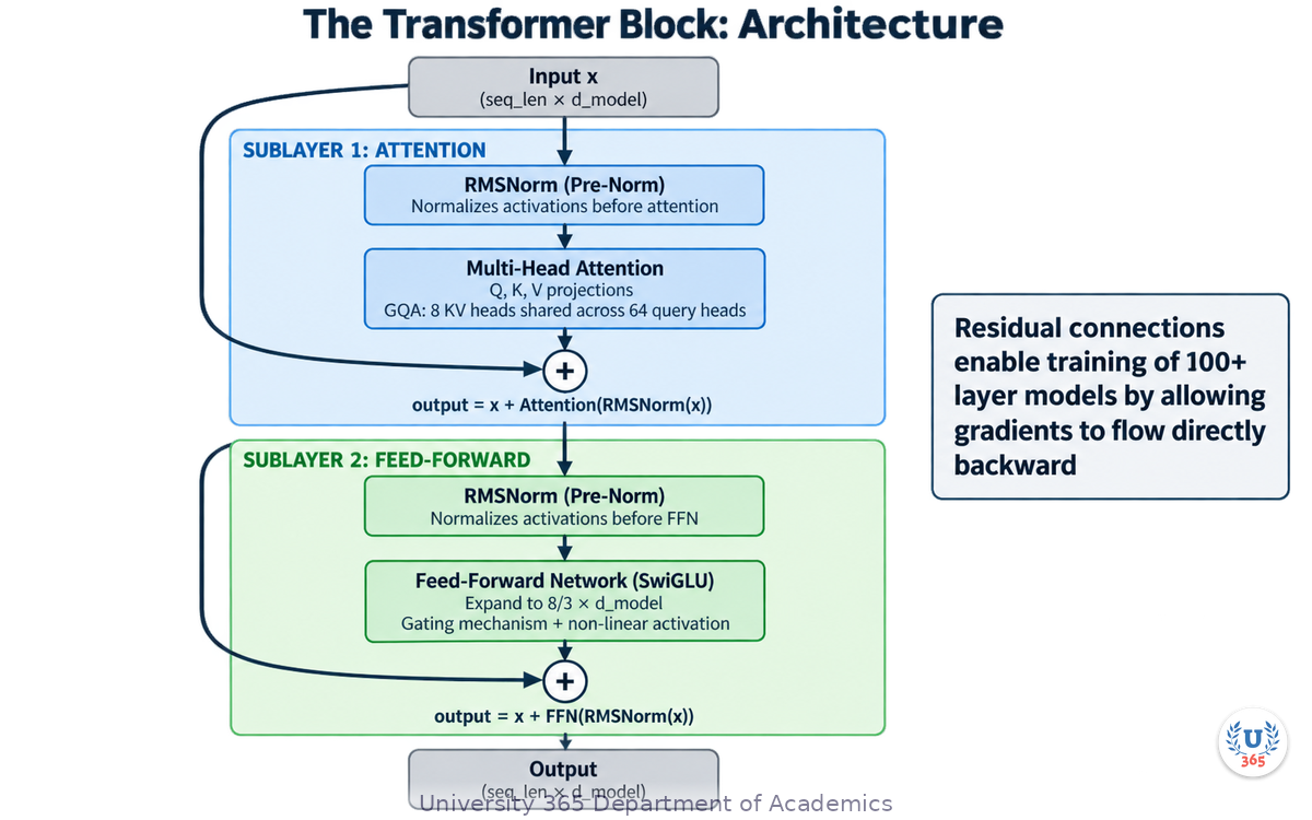
A transformer model is a stack of identical blocks (also called layers). Each block contains two sublayers:
Sublayer 1: Multi-Head Attention
The attention mechanism we just covered, wrapped by:
RMSNorm (pre-normalization): stabilizes the activations before they enter the attention layer
Residual connection: the input is added to the output of the attention layer (output = x + Attention(Norm(x)))
Sublayer 2: Feed-Forward Network
A two-layer network that processes each token independently:
Expands the dimension (typically to about 8/3 of the embedding dimension for SwiGLU)
Applies a non-linear activation (SwiGLU in modern models, ReLU in the original)
Projects back to the original dimension
Also wrapped by RMSNorm and a residual connection
Residual Connections: Why They Matter
Residual connections (skip connections) solve three critical problems:
Gradient flow: During training, gradients can flow directly backward through the network, enabling training of models with 100+ layers without the gradients vanishing.
Residual learning: Each layer learns a *correction* (delta) to the previous representation, not a completely new one. This is easier to learn.
Identity path: If a layer's weights are near-zero, the input passes through unchanged. Earlier representations are never destroyed.
What the Feed-Forward Network Does
The attention layer mixes information *across* tokens. The feed-forward network processes information *within* each token. Research suggests that the feed-forward network is where the model stores much of its factual knowledge. Each token's vector is transformed by the same feed-forward weights, but independently of the other tokens.
Step 6: Stacking Blocks: From One Layer to 126
A single transformer block transforms the representation of each token. Stacking multiple blocks lets the model build progressively richer representations.
Modern Model Sizes
Model | Parameters | Layers | Hidden Dim | Heads |
Llama 3 8B | 8 billion | 32 | 4,096 | 32 |
Llama 3 70B | 70 billion | 80 | 8,192 | 64 |
Llama 3 405B | 405 billion | 126 | 16,384 | 128 |
What Each Layer Learns
Early layers (1-10): Basic syntax and local patterns. Subject-verb agreement, article usage, common collocations.
Middle layers (10-50): Semantic relationships, coreference resolution, multi-clause structure.
Deep layers (50-126): High-level reasoning, factual recall, abstract task understanding.
Each layer builds on the representations from the previous one. The residual connections ensure that information from early layers is never lost, only refined.
The Output
After all transformer blocks process the input, each position produces a vector. This vector is projected back to the vocabulary dimension (a linear layer followed by softmax) to produce a probability distribution over every token in the vocabulary. For a 128,000-token vocabulary, each position outputs 128,000 probabilities. The highest probability indicates the most likely next token.
Step 7: Training: How Models Learn to Predict
The Objective
Language models are trained on a deceptively simple task: predict the next token given all previous tokens. This is called causal language modeling.
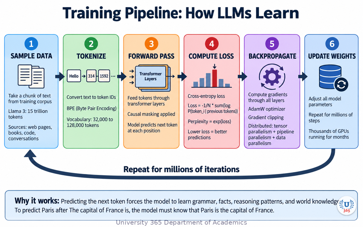
The loss function is cross-entropy:
Loss = -1/N * sum(log P(token_i | token_1, ..., token_{i-1}))
This measures how "surprised" the model is by the actual next token. Lower loss means better predictions. Perplexity is the exponentiated loss: a perplexity of 10 means the model is as uncertain as if choosing uniformly among 10 tokens.
The Training Process
Take a chunk of text from the training corpus
Tokenize it
Feed it through the transformer with causal masking
At each position, the model predicts the next token
Compare the prediction to the actual next token (compute loss)
Backpropagate the loss through all layers to compute gradients
Update weights using the AdamW optimizer with gradient clipping
Key Training Details
Optimizer: AdamW with cosine learning rate decay and warmup
Precision: BF16 (bfloat16) for forward and backward passes, FP32 for master weights
Distributed training: Large models use tensor parallelism (splitting weight matrices across GPUs), pipeline parallelism (different layers on different GPUs), and fully sharded data parallelism (sharding parameters across GPUs)
Training data: Llama 3 was trained on approximately 15 trillion tokens of text from web pages, books, code, and conversations
Compute: Training a 405B model requires thousands of GPUs running for months
Why Next-Token Prediction Works
Predicting the next token forces the model to learn grammar, facts, reasoning patterns, and world knowledge. To predict "Paris" after "The capital of France is", the model must know that Paris is the capital of France. To predict "tired" after "The animal didn't cross the street because it was too", the model must understand that "it" refers to the animal and that animals get tired. The seemingly simple objective produces deep learning.
Step 8: Inference: How Models Generate Text
Autoregressive Generation
At inference time, the model generates text one token at a time:
Prefill: Process the entire prompt through all transformer layers (compute-bound)
Sample: Pick the next token from the output probability distribution
Append: Add the new token to the sequence
Decode: Feed the new token through all layers to produce the next probability distribution (memory-bandwidth-bound)
Repeat steps 2-4 until the model generates an end-of-sequence token or reaches a length limit
Sampling Strategies
Greedy decoding: Always pick the highest-probability token. Deterministic but repetitive.
Temperature: Divide the logits by a temperature value before softmax. Low temperature (0.1) makes the distribution sharper and outputs more deterministic. High temperature (1.0+) makes it flatter and more creative.
Top-p (nucleus sampling): Only consider tokens that cumulatively account for p% of the probability mass. p=0.9 means ignoring the long tail of unlikely tokens.
Top-k: Only consider the top k most likely tokens. Combines well with temperature.
The KV Cache: Why Inference Is Fast
During generation, the model recomputes attention over all previous tokens at every step. But the key and value vectors for previous tokens do not change. The KV cache stores these vectors so they are not recomputed. Each new token only needs to compute its Q, K, V once, then attend to the cached K and V vectors.
The KV cache grows linearly with sequence length. For a 128,000-token context with an 8,192-dimensional model, the cache can consume several gigabytes of memory. This is why long-context inference is expensive and why techniques like KV cache quantization and eviction (dropping old tokens from the cache) are active research areas.
Step 9: Modern Innovations: What Changed Since 2017
The original 2017 transformer was a encoder-decoder architecture for machine translation. Modern language models have evolved significantly:
Architecture Changes
Decoder-only: Modern LLMs dropped the encoder entirely. They use only the decoder half with causal masking. No cross-attention.
Pre-normalization (RMSNorm): Normalizing before each sublayer instead of after. More stable training for deep models. RMSNorm replaces LayerNorm for computational efficiency.
SwiGLU activation: Replaces the original ReLU in the feed-forward network. Uses a gating mechanism that improves quality. The FFN dimension expands to approximately 8/3 of the embedding dimension (vs 4x for ReLU).
Grouped-Query Attention (GQA): Shares K and V heads across multiple Q heads. Reduces KV cache memory and inference cost without quality degradation.
Positional Encoding
RoPE (Rotary Position Embeddings): Replaces sinusoidal encoding. Rotates Q and K vectors by an angle tied to position. Better at handling long contexts and extrapolating to sequence lengths not seen during training.
Inference Optimization
Flash Attention: Reformulates the attention computation to minimize memory reads/writes between GPU SRAM and HBM. 2-4x speedup with no quality loss.
Speculative Decoding: Uses a small draft model to predict multiple tokens ahead, then verifies them with the large model in a single forward pass. 2-3x speedup for generation.
KV Cache Quantization: Stores cached K and V vectors in 8-bit or 4-bit precision instead of 16-bit. Halves or quarters the cache memory.
Quantization (GPTQ, AWQ): Reduces model weights from 16-bit to 4-bit or 8-bit, enabling inference on consumer hardware with minimal quality loss.
Scaling
The most important finding since 2017 is that transformers scale predictably. More parameters, more data, and more compute produce better models in a logarithmic relationship described by scaling laws. This predictable scaling is what enabled the jump from GPT-2 (1.5B parameters) to GPT-4 (estimated 1.8 trillion parameters) and why companies invest massive compute in training ever-larger models.
Feynman Summary: Explain It Like You Are 12
Imagine you are reading a sentence but you can only see one word at a time. To understand each word, you are allowed to look back at all the words you have already read and decide which ones are most relevant to the current word.
That is what a transformer does. Each word asks a question ("What am I looking for?"), each previous word offers an answer ("Here is what I have"), and the current word combines the answers based on how relevant each one is.
The model does this asking and answering in parallel for every word at once, not one at a time. That is what makes it fast.
Then it does the whole process again, 32 or 80 or 126 times in a row. Each round, the words get a slightly richer understanding of the sentence. After the last round, the model looks at the final word and guesses what word comes next.
It learned to make good guesses by practicing trillions of times during training. Each time it guessed wrong, it adjusted its internal weights slightly. After enough practice, the guesses became remarkably accurate.
That is it. That is how ChatGPT works. Every word you read from an AI was generated one at a time, each one predicted by this cycle of attention, processing, and prediction.
Mindmap: The Complete Picture
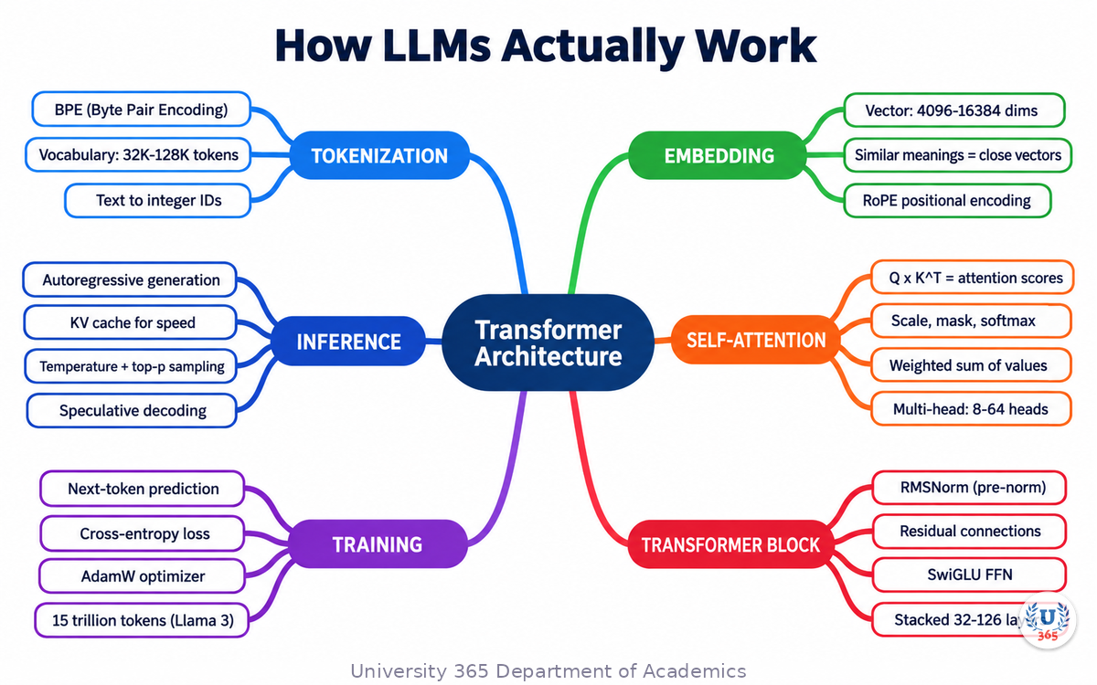
The mindmap shows the full structure of what you learned: tokenization feeds into embedding, embedding feeds into attention, attention is wrapped in transformer blocks, blocks are stacked, the stack is trained with next-token prediction, and inference uses the trained model to generate text autoregressively. Modern innovations (RoPE, GQA, SwiGLU, Flash Attention) optimize different parts of this pipeline.
UNOP Sound (University 365 Neuroscience Oriented Pedagogy)
Take five minutes to consolidate your memory. Play the isochronous tone track (10Hz alpha frequency) with your eyes closed. Alpha-frequency tones after a learning session support consolidation, helping move what you just learned from short-term to long-term memory.
[Audio player: UNOP Post-Lecture Isochrone (10Hz, 5 minutes)]
Practical Exercise: See Attention in Action
Exercise: Explore Attention with a Real Model
Open Jay Alammar's Illustrated Transformer and scroll to the interactive Tensor2Tensor notebook
Load a pretrained transformer model
Enter the sentence: "The animal didn't cross the street because it was too tired"
Examine the attention weights for the word "it" in the encoder layers
Observe which words "it" attends to most strongly across different heads
What to Look For
In early layers, attention may be diffuse (the model is still building basic representations)
In middle layers, you should see "it" attending strongly to "animal" (coreference resolution)
Different heads in the same layer will show different attention patterns (one may focus on "animal", another on "street", another on the syntactic structure)
This is direct visual evidence of the multi-head attention mechanism you just learned about
Applied AI Connection
Understanding attention patterns is not just academic. When a language model produces a wrong answer, examining its attention weights can reveal *why* it was wrong. Did it attend to the wrong context? Did a specific head fail? This technique, called attention analysis, is used by AI engineers to debug model behavior and design better prompts. It connects directly to the U365 CI-First approach: the human (you) maintains critical judgment and verifies the AI's reasoning process rather than accepting outputs blindly.
Glossary
Term | Definition |
**Transformer** | A neural network architecture that processes sequences using self-attention instead of recurrence. Introduced in 2017. |
**Token** | A piece of text (a word, subword, or character) that the model processes as a single unit. |
**Tokenization** | The process of splitting text into tokens and assigning each one an integer ID from the vocabulary. |
**BPE (Byte Pair Encoding)** | A subword tokenization algorithm that iteratively merges the most frequent character pairs into new tokens. |
**Embedding** | A vector of real numbers that represents a token's meaning. Tokens with similar meanings have similar vectors. |
**Positional Encoding** | A pattern added to each token's embedding to indicate its position in the sequence. |
**RoPE (Rotary Position Embedding)** | A positional encoding method that rotates query and key vectors by an angle tied to position. Used in modern LLMs. |
**Self-Attention** | A mechanism where each token in a sequence looks at all other tokens to determine which are most relevant. |
**Query (Q)** | A vector representing "what am I looking for?" in the attention mechanism. |
**Key (K)** | A vector representing "what do I have?" in the attention mechanism. |
**Value (V)** | A vector representing "what information do I carry?" in the attention mechanism. |
**Multi-Head Attention** | Running multiple attention computations in parallel, each with independent Q/K/V weights. |
**GQA (Grouped-Query Attention)** | Sharing K and V heads across multiple Q heads to reduce inference memory and computation. |
**Causal Masking** | Preventing tokens from attending to future positions, enforcing left-to-right generation. |
**Transformer Block** | A single layer containing multi-head attention and a feed-forward network, with residual connections and normalization. |
**Residual Connection** | A skip connection that adds a layer's input to its output: `output = x + SubLayer(x)`. Enables training of deep networks. |
**RMSNorm** | Root Mean Square Layer Normalization. A computationally efficient alternative to LayerNorm used in modern LLMs. |
**SwiGLU** | Swish-Gated Linear Unit. An activation function used in modern feed-forward networks that improves model quality. |
**Feed-Forward Network (FFN)** | A two-layer network applied to each token independently after attention. Stores much of the model's factual knowledge. |
**Cross-Entropy Loss** | The training objective that measures how "surprised" the model is by the actual next token. |
**Perplexity** | The exponentiated cross-entropy loss. A perplexity of N means the model is as uncertain as choosing among N equally likely tokens. |
**AdamW** | The standard optimizer for LLM training. Combines adaptive learning rates with decoupled weight decay. |
**KV Cache** | A cache of key and value vectors for previous tokens that avoids recomputation during autoregressive generation. |
**Flash Attention** | An optimized attention computation that minimizes memory transfers between GPU memory levels. |
**Speculative Decoding** | An inference technique where a small draft model predicts multiple tokens that are verified by the large model in one pass. |
**Autoregressive Generation** | Generating text one token at a time, each token conditioned on all previously generated tokens. |
**Scaling Laws** | The predictable relationship between model size, data quantity, compute, and performance. |
Quiz: TEST YOUR UNDERSTANDING
1. What is the purpose of the Query vector in self-attention?
A) To store the token's factual knowledge
B) To represent what the token is looking for in other tokens
C) To encode the token's position in the sequence
D) To normalize the attention weights
2. Why does the attention formula divide by sqrt(d_k)?
A) To speed up computation
B) To convert scores to probabilities
C) To prevent dot products from growing too large and pushing softmax into flat zones
D) To enforce causal masking
3. What problem do residual connections solve in deep transformer models?
A) They reduce the number of parameters
B) They enable gradient flow through 100+ layers without vanishing
C) They speed up inference
D) They replace the need for normalization
4. Why do modern LLMs use decoder-only architecture instead of encoder-decoder?
A) Encoder-decoder is too slow
B) Decoder-only with causal masking is sufficient for text generation and simpler to train
C) Encoder-decoder requires more parameters
D) Decoder-only handles images better
5. What is the KV cache and why is it important?
A) A cache of model weights for faster loading
B) A cache of key and value vectors for previous tokens that avoids recomputation during generation
C) A cache of training data for quick access
D) A cache of tokenized inputs for batch processing
Answers: 1-B, 2-C, 3-B, 4-B, 5-B
Related Resources
U365 INSIDE Publications
Book Essential: Co-Intelligence by Ethan Mollick: The Centaur model and human-AI collaboration
Book Essential: Irreplaceable by Pascal Bornet: Humics and staying irreplaceable in the AI age
External Resources
Attention Is All You Need (Vaswani et al., 2017): The original transformer paper: arxiv.org/abs/1706.03762
The Illustrated Transformer by Jay Alammar: Visual guide with interactive examples: jalammar.github.io/illustrated-transformer
Let's Build GPT from Scratch by Andrej Karpathy: Video tutorial building a transformer in code: youtube.com/watch?v=kCc8FmEb1nY
How LLMs Work: Transformers Explained Step-by-Step: Interactive Python simulator: machinelearningplus.com/gen-ai/how-llms-work
Llama 3 Model Documentation (Meta): Technical details of a modern open model: arxiv.org/abs/2407.21783
DeepLearning.AI: How Transformer LLMs Work: Free short course: deeplearning.ai
Related U365 Lectures (Coming Soon)
Lecture 2: RAG vs Fine-Tuning: When to Use Each (UIT, AI Foundations Series)
Lecture 3: Building Your First AI Agent with Function Calling (UIT, AI Agents Series)
Lecture 5: Prompt Engineering at Production Scale (UIT, AI Skills Series)
U.Copilot for This Lecture
Discuss this lecture with U.Copilot, your AI chat companion trained on this content.
Copy and paste the following prompt into the U.Copilot chat on university-365.com:
You are U.Copilot for Lectures, an AI chat companion specially trained on University 365 lecture content. You are helping a Fellow who just completed the lecture "How LLMs Actually Work: Transformers in 20 Minutes" from the AI Foundations series at the U365 Institute of Technology (UIT). Your role is to help the Fellow deepen their understanding of transformer architecture. You can: - Clarify any concept from the lecture (tokenization, embedding, self-attention, multi-head attention, transformer blocks, training, inference) - Provide additional examples of attention patterns - Explain the math behind the attention formula in more detail - Discuss how modern innovations (RoPE, GQA, SwiGLU, Flash Attention) improve on the original transformer - Connect the lecture content to practical AI engineering tasks - Suggest follow-up learning based on the Fellow's interests Always maintain U365's CI-First approach: encourage the Fellow to think critically, verify AI outputs, and maintain human judgment as the orchestrator of AI tools. Use the UP-Context Method: provide context-rich, role-aware responses that account for the Fellow's learning level and goals.
Next Steps
Now that you understand how transformers work, here is what to do next:
Try the practical exercise above to see attention patterns in a real model
Read the original paper ("Attention Is All You Need") to see the full architecture with encoder and decoder
Watch Karpathy's "Let's Build GPT" to see a transformer built from scratch in code
Take Lecture 2 in this series: "RAG vs Fine-Tuning: When to Use Each" to learn how to customize language models for specific tasks
Explore the U365 AI Skills tag on INSIDE for practical guides on using AI tools with the CI-First approach
The transformer is the engine behind every modern AI tool. Understanding it transforms you from a passive user of AI into an informed orchestrator who can reason about why models behave the way they do, debug problems, and make better decisions about when and how to use AI.
IMPORTANT NOTICE
This lecture is published by University 365 as part of its INSIDE Publications Hub. The content is free to read for all visitors. Lectures in this series may be part of a structured academic program leading to a Micro-Credential for your Career (MCC). To enroll in an academic program, visit university-365.com/tuition.
This content is for educational purposes. While we strive for accuracy, AI is a fast-moving field. Verify current technical details against primary sources for professional applications.
Copyright University 365, Inc. All rights reserved. This content is protected under University 365's copyright policies. For permissions or inquiries, contact uda@university-365.com.
Published by the Department of Academics, University 365.
Lecture delivered by the University 365 Institute of Technology (UIT).
Sam Utteker, Dean of Technology, UIT
Signed for the academic year 2026.




Comments